


JP Vasseur1 (jpv@cisco.com), PhD - Fellow/VP; Gregory Mermoud1 (gmermoud@cisco.com), PhD – Distinguished Engineer; PA Savalle1 (psavalle@cisco.com), PhD – Principal Engineer; Eduard Schornig1 (eschornig@cisco.com) – Principal Engineer; Mukund Yelahanka Raghuprasad1 (myelahan@cisco.com) – Technical Leader; Andrea Di Pietro (andipiet@cisco.com), PhD - Technical Leader; Gregoire Magendie (gmagendie@cisco.com) - Senior Software Engineer; Romain Kakko-Chiloff - Senior Software Engineer (rkakkoch@cisco.com).
1All authors are affiliated with Cisco Systems.
Release v1 – August 2023
Challenging the Norm: A Groundbreaking Experiment in AI-Driven Quality of Experience (QoE) with Cognitive Networks
Abstract: Quality of Experience (QoE) is arguably the most critical indicator of networking performance. For the past three decades, QoE has been measured using network-centric variables such as path delay, loss, and jitter, with hard-coded bounds that should not be exceeded. In this study, we take a radically different and novel approach by gathering a rich set of cross-layer variables across the stack, along with real-time a large number of user feedback (binary flag), to train a Machine Learning (ML) model capable of assessing and learning the true user experience (QoE). We trained various ML models, such as GBTs and Attention Models, which showed highly interesting and promising results. We also propose a strategy to extend such models to different domains (applications) using transfer learning. We demonstrate that it is indeed possible to learn the complex network phenomenon that drive actual QoE, which could be integrated into future networking approaches for QoE visibility and potentially Self-Healing networks driven by QoE. This approach could enable a radically different set of network design principles, governed by an objective function centered around application or user QoE, as opposed to traditional networking characteristics such as bandwidth, delay, and loss, which so far have been poorly mapped to QoE other than with static thresholds. This method could be used not only to measure QoE effectively but also to trigger automation and build future self-healing networks that constantly optimize themselves to enhance QoE.
1. Disrupting a 20-year-old network-centric vision of QoE
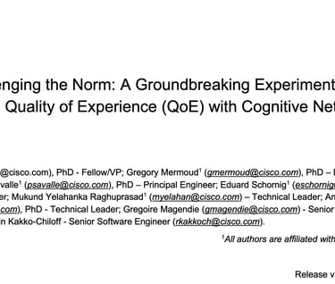
Since the late 1990s a plethora of tools have been developed and deployed at scale to measure various network characteristics at multiple layers. SNMP and the newer Model Driven Telemetry (MDT) are widely used to monitor link layer characteristics such availability, error rates, buffers, QoS drops while OAM PM (Y.1731) and MPLS PM (& SR PM) have been long used to monitor performance of ethernet or MPLS services in Service Provider networks. At the IP layer there are plenty of options available, from standardized protocols (TWAMP, OWAMP) to vendor specific functionality (Cisco's IP SLA, Juniper's RPM) that achieve a similar function of monitoring loss, latency, and jitter. Higher up in the stack at the transport and application layers, tools such as Cisco's ART & Perf Monitor running on network devices and a variety of Real User Monitoring (RUM) tools embedded into the application or deployed as agents on end user devices can be used to collect rich sets of end-to-end performance metrics.
The Internet Engineering Task Force (IETF, https://www.ietf.org/) has published several RFCs such as RFC4594 (https://datatracker.ietf.org/doc/html/rfc4594) that specifies several services classes and how they can be used with Differentiate Services (DiffServ), traffic conditioners and queueing mechanisms. The document also proposes for each service class (e.g. Network control, telephony, signaling, Multimedia conferencing, etc.) quantitative values that indicate the sensitivity of the various classes of traffic to networking characteristics such as the Loss, Delay and Jitter (from very Low to High). Over the years rough consensus have emerged that “specifies” hard values that should not be exceeded to preserve the user Quality of Service (QoS). For example, a commonly adopted set of values for Voice/Video (real-time) are:
· Max Delay (one way): 150ms
· Max Jitter: 50ms
· Max Packet Loss rate: 3%
1.1 The under-specification of measurements granularities
The measurements granularity is usually left unspecified making the values much less relevant. A path experiencing a constant delay of 120ms for voice over a period of 10 minutes provides a very different user experience than a path with the same average delay that keeps varying between 20 and 450ms during the same period… The dynamics of such KPIs are even more critical for packet loss and jitter in the case of voice and video traffic (e.g., 10s of 80% packet loss would severely impact the user experience although averaged out over 10’ the average would show a low value, totally acceptable according to the threshold).
Without a doubt, the user experience requires a more subtle and accurate approach to determine the networking requirements a path should meet to maximize the user satisfaction (QoE). Such an approach must be capable of understanding patterns that impact QoE, which as shown later in this document are more complex than computing averages for Loss, Delay and Jitte. It may also be beneficial to take into account telemetry from upper layers (applications) and capture local phenomenon (e.g. effects on delay, jitter and loss at higher frequencies as discussed in (Vasseur, Mermoud , Schornig, Raghuprasad, & Magendie, 2023)
1.2 Application scores
The most common approach to assess QoE is either to consider whether Service Level Agreement (SLA) is met and/or to keep track of application health scores. Such scores are usually ranked between 1 and n (with n=5 or 10) where higher scores correspond to better user QoE. Still, how should such score be computed is left to the implementer.
For the most part, scores are computed as linear combinations of other more-specific scores mostly related to network performance. The result is an overall (highly) aggregated value that reflects QoE (per user, per application, aggregated across users in a location, etc.). Weights used in such formulas are not learned based on user feedback but rather tuned using iterative approaches (sometimes) driven by user survey campaigns. An example of such an application score that we will use extensively in this study is the Webex User Experience Score (UES), which is a heuristic crafted by experts based on L3 and L7 metrics (loss, RTT, concealment times, etc.).
In contrast, Cognitive Networks make use of Machine Learning (ML) to compute the QoE as a probability for the user to have a “Good” experience where labels (user feedback) are collected, and the ML algorithm automatically learns complex patterns that drives the user experience.
1.3 On layer violation
For years, the concept of layers isolation has been a core principle of the Internet. Such an approach allowed for avoiding dependency between layers at a time where several protocols and technologies were developed at each layer. Such an approach has proven to be quite effective in enabling the design and deployment of new protocols at different layers (e.g., PHY, MAC, …) independent of each other, allowing the Internet to scale. However, this approach has several shortcomings, not the least of which is the difficulty of optimizing objective functions across layers.
Still, with modern applications requiring tight SLAs a cross-layer approach is highly desirable. Although a strict layer-isolation approach has been quite effective the effect of specific actions at a given layer of the networking stack on user experience are qualitatively evaluated, but being able to precisely quantify is much harder: determining that voice quality is low along a highly congested path may be relatively easy but by how much should the bandwidth be increased or how should the weight of the queue used for voice be tuned in order to increase the user experience score? The use of (ML) models allows for such quantification.
2 Introducing the concept of “Cognitive” Networks
Cognition is defined as "the mental action or process of acquiring knowledge and understanding through thought, experience, and the senses." It encompasses various intellectual functions and processes, including perception, attention, thought, intelligence, knowledge formation, memory, working memory, judgment, evaluation, reasoning, computation, problem-solving, decision-making, and both comprehension and production of language. Imagination is also considered a cognitive process because it involves contemplating possibilities. Cognitive processes utilize existing knowledge and facilitate the discovery of new knowledge.
Cognitive (from the Latin noun cognitio, i.e., 'examination,' 'learning,' or 'knowledge') functions in the brain correspond to the mental processes enabling a broad range of intellectual functions such as learning (knowledge), attention, thoughts, reasoning, language and understanding of the world. In neuroscience, cognition is a sub-discipline focusing on the study of the underlying biological processes of cognition with a core focus on neuronal activities.
Cognitive Networks refer to the ability of acquiring knowledge (QoE measured from user feedback, KPIs at all layers) and understanding (learning) what drives the QoE, using ML/AI algorithms capable of predicting QoE according to the various variables of the stack.
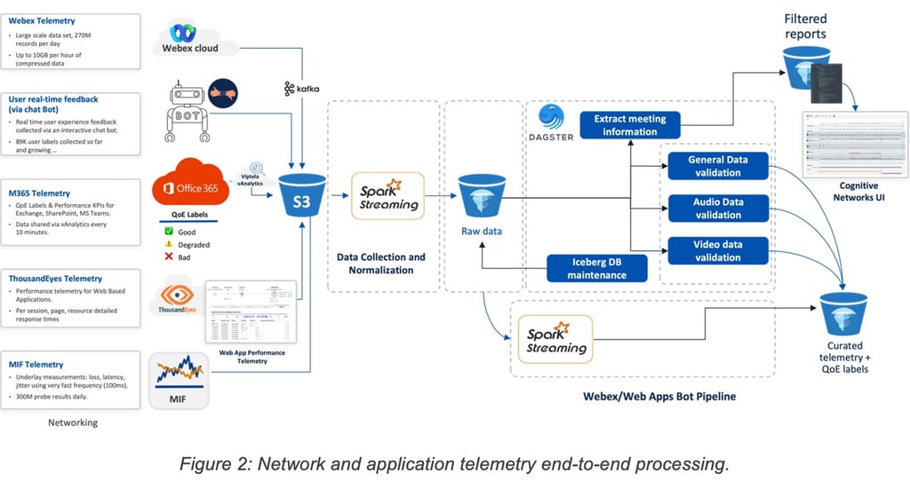
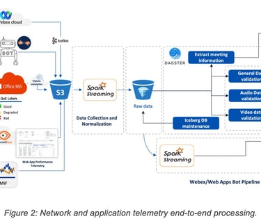
2.1 Gathering cross-layer telemetry
In the context of Cognitive Networks, multiple such sources of telemetry can be used:
§ Application: in the context of our experiment, rich Webex media quality reports are produced for each meeting participant at 1-minute granularity containing hundreds of KPIs that capture detailed information about network and application performance. An example of a few of the KPIs recorded:
Layer 3 metrics:
Latency (avg, max RTT)
Loss (end-to-end, hop-by-hop)
Jitter (end-to-end, hop-by-hop)
Bitrates (transmitted/received)
Layer 7 metrics (audio, video, content sharing):
Concealment Time
Jitter Buffer
Video Resolutions (requested, received)
Framerates
Codec type
Microsoft Office365: reports are produced every 10 minutes at circuit level (public IP address) for 3 application categories: Teams, Exchange, SharePoint. Each report contains:
Application quality label: “Good”, “Degraded”, “Bad”, “No Opinion”.
Aggregated network performance metrics: latency, jitter, packet loss, bandwidth usage.
Advanced Probing system (e.g., ThousandEyes): Enterprise Agents have been deployed on end-user hosts and allowed to monitor browser-based application performance. Here are a few examples of metrics recorded:
Host device metrics: CPU usage, Memory usage, device type, connection type (wired, WiFi)
Network metrics: WiFi Quality, Packet Loss, Latency, Jitter, Hob by Hop network path (traceroute)
HTTP Archive (HAR) telemetry: DNS, TCP, SSL timers, HTTP errors, page and resource load and response times
High Granularity Telemetry: The MIF agent (as discussed in (Vasseur J. , Mermoud , Schornig, Raghuprasad, & Magendie, 2023)) is a synthetic probing agent that enables network monitoring (loss, latency, jitter) at very fast frequencies (100ms) allowing detection of short-lived network events that would otherwise go undetected.
2.2 Gathering offline user feedback using crowd sourcing
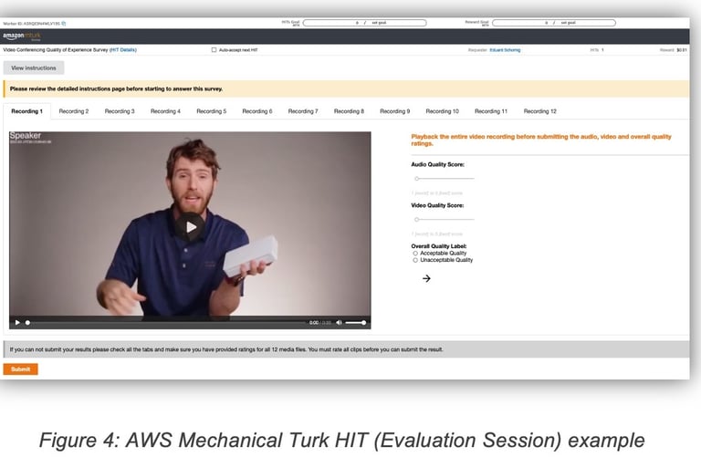
One approach to understanding the effect of various types of network degradations on the perceived user experience consists in collecting real user feedback using a crowd-sourced data labeling platform like AWS Mechanical Turk (denoted MTurk hereafter).
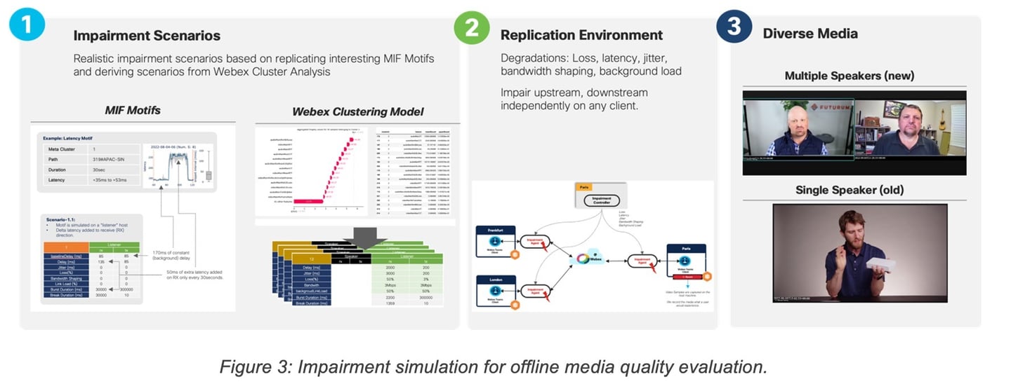
To this end, a dedicated environment was built where different types of collaboration clients (Webex, MS Teams, Zoom) were instantiated and configured to join audio/video conferences. At the same time, impairment agents were used to intercept the application traffic and inject various representative patterns of degradations (loss, latency, jitter, bandwidth restrictions) on one or more participants. The impairment patterns used corresponded to frequent types of degradations captured previously by either MIF telemetry or Webex telemetry (see Figure 3).
The resulting media (audio/video) was recorded and submitted for evaluation by human users via the MTurk platform. Participants were asked to rate the quality of the media using two types of scores:
1 (worse) to 5 (best) score for audio and video (independently)
Acceptable/Unacceptable Quality
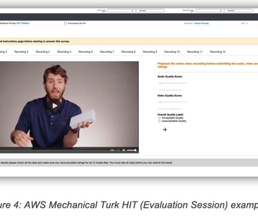
To keep the quality of the received feedbacks high and eliminate feedbacks from inattentive users or users providing random answers, two control mechanisms were used. First, MTurk users had to already achieve a set of worker qualification metrics (Number of Completed HITs > 5000, % of approved HITs > 99%, Worker is an MTurk Master) indicating a good reputation on the platform before they can start answering QoE related HITs. A second control mechanism consists in including so-called baseline samples, i.e. known good (no degradation, perfect audio and video) and known bad (major degradation, severe degradation of video and audio) media files, in each evaluation session. Users that rate baseline media samples incorrectly are excluded from further analysis.
Several QoE feedback campaigns were conducted leading to more than 10K labels being collected.
2.3 Gathering real-time user feedback using a Webex Bot
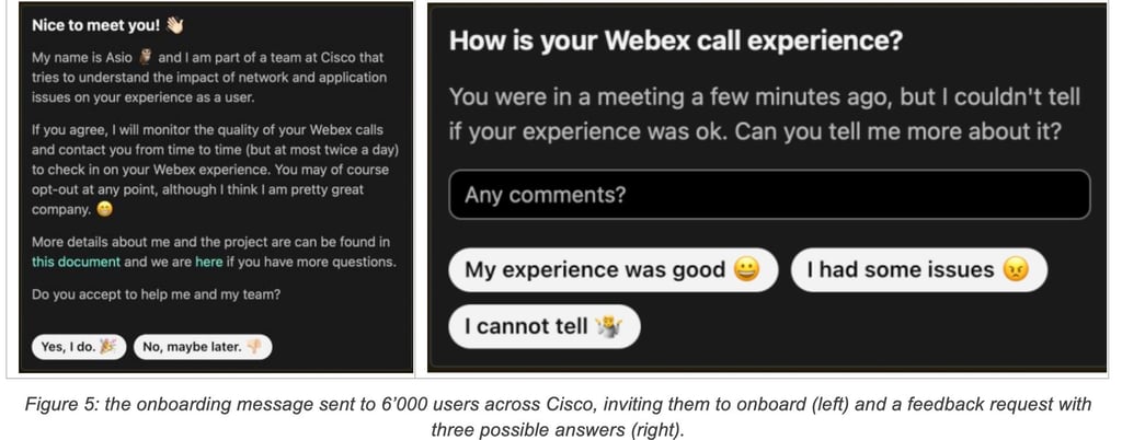
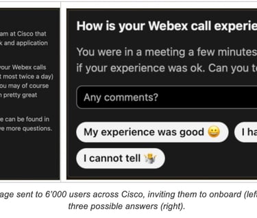
Gathering user feedback was an essential component of the Cognitive Networks experiment. The experiment lasted for a duration of three months thanks to the collaboration of 6,000 users providing max 2 feedback every day, leading to a total of 100K labels associated with a rich set of cross-layer telemetry as discussed above.
To be able to collect feedback at such scale, the Webex bot had to perform two distinct functionalities:
1. Given a set of candidate participants to the project, ask each one of them to opt in or out.
2. Request timely feedback under relevant network conditions to users who opted in.
To this end, the bot system was made up of two main components:
1. A back-end server, responsible for probing a set of candidate users and performing feedback requests.
2. A combination of streaming pipelines responsible for consuming and analyzing the Webex telemetry for every user participating to the project and determining when to request feedback.
The back-end server was provided with large lists of candidate users and would contact each one of them via the Webex Teams chat. Users would receive a request describing the goal of the project and would be asked whether they agreed to provide their feedback (an example is provided in Figure 5). The response for each user was stored into a back-end database and used to determine whether to send feedback requests. It was possible for each user to change his decision at any time by sending specific chat messages to the back end.
When the streaming pipeline determines that feedback should be requested for a given user, it sends a request to the back-end server. In turn, the back-end server checks the user opt-in status and applies a rate limiting mechanism (which will be described in greater detail later). If the feedback request passed both checks, the back-end server sent a chat message to the user asking about their perceived experience. Upon receiving the user response, the back-end server appended it to the dataset.
The back end was also responsible for collecting “unsolicited feedback”: users who opted-in could spontaneously provide feedback about their experience during a Webex call, by sending a message to the chat bot. Such feedback was always added to the data set without being subjected to any filtering mechanism.
As mentioned, the goal of the streaming pipeline was to monitor the Webex telemetry and to decide when to send a request to the end user. Such request was triggered by specific network conditions. To make sure that the user feedback would be as close as possible to the actual network condition of interest (e.g., packet loss), reducing the feedback request delay was crucial. This was an important requirement in driving the design of the pipelines.
To this end, the bot largely relied on stream processing technologies for processing a large amount of telemetry data with a bounded and low latency. More precisely, the Apache Spark structured streaming technology has been leveraged for big data processing in near real time. Such design allowed the delay between the triggering event and the feedback collection to be in the order of a few minutes in most cases.
A first streaming pipeline oversaw the ingestion of the Webex telemetry for the target organization. Detailed reports for each call at a one-minute granularity would be received and stored into an Apache Iceberg table.
A second pipeline oversaw the processing of the data as they landed in the Iceberg table:
1. Filter telemetry samples for potentially onboarded users (all other samples were ignored).
2. For each telemetry sample, make a decision of whether a feedback request should be sent.
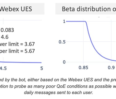
In particular, the decision to request a user feedback was made based on a sampling probability that is derived using the QoE estimates for the user. Considering that examples of degraded QoE are relatively rare, the sampling probability was biased towards poor QoE estimates. This ensures collection of a diverse set of samples corresponding to the various types of QoE degradations (see Figure 6).
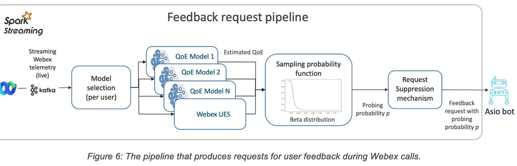
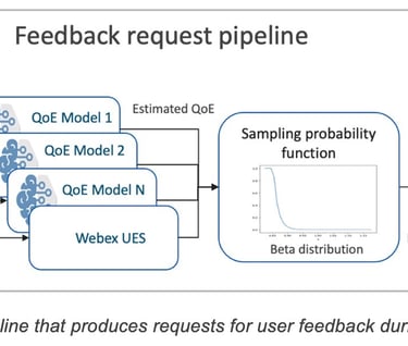
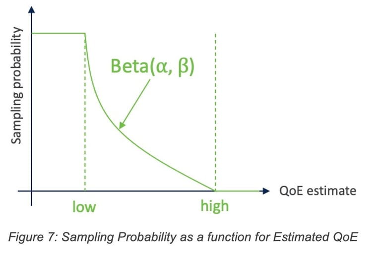
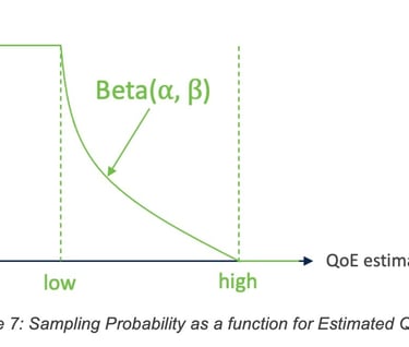
The sampling probability is a beta-distribution that is fit on the QoE estimate as the random variable. The lower the QoE estimate for some telemetry, the higher is the corresponding sampling probability. For a given QoE estimate, the beta distribution parameters low, high, ⍺, and β are optimized using Bayesian optimization (hyper-opt). The objective for the optimization is to achieve the lowest “sampled” QoE estimate, with the constraint that average number of feedback requests per user, per day falls in the range of [1.0, 1.5] requests.
Sampling strategies differ primarily in the QoE estimate that is used to derive the sampling probability. We studied two strategies, one relying on the Webex UES and the other relying on model predictions as QoE estimators. The beta distribution parameters were optimized for both strategies using the same data and constraints mentioned above. The optimized beta distributions for Webex UES and predicted QoE were as shown in Figure 8.
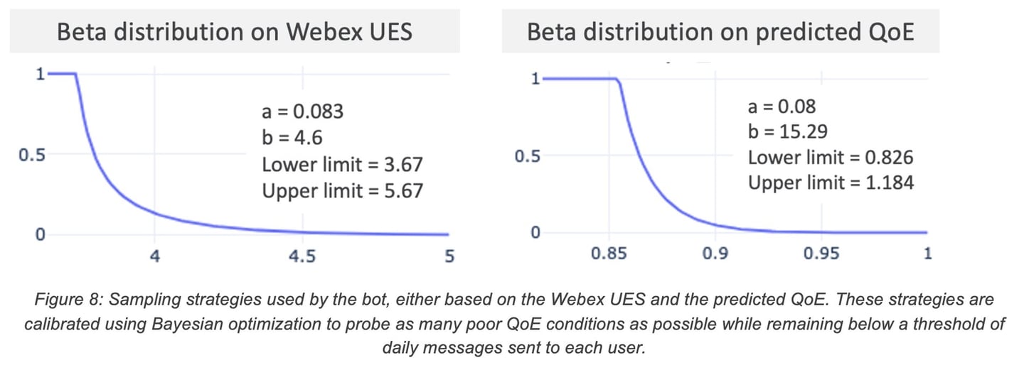
Considering that the sampling strategy is targeted towards obtaining the maximum number of samples that correspond to negative feedback (user “unhappy”), the percentage of total feedbacks that correspond to negative QoE can be used to measure the performance of a sampling strategy. This measure also called the “negativity rate” measures the effectiveness of a sampling strategy along with the “response rate”, which measures that percentage of users that responded to a feedback request. The two strategies above were A/B tested among two randomly chosen groups of users. Response rates for both the strategies were approximately 35%, the negativity rate for the strategy using predicted QoE was measured at 8.5% while the strategy using Webex UES was measured at 6.6%. This implies that the QoE predicted by our QoE models may serve as a better indicator of QoE degradation compared to Webex UES.
To make sure that the number of feedback requests per user did not exceed the quota that has been advertised upon project opt-in, a safety mechanism has been integrated in the back end. Upon receiving each feedback request from the pipeline, the back-end server checks the message history sent to the target user and ignores the request if the quota is exceeded.
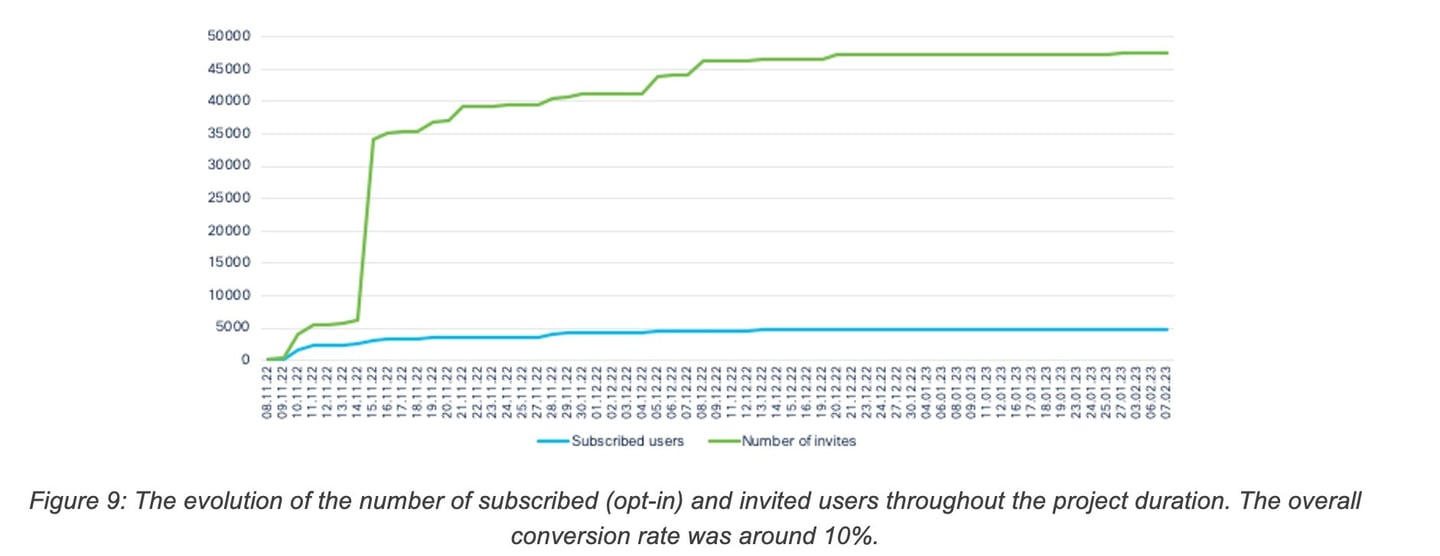
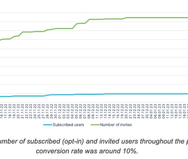
To build a large community of users and to collect a diverse and large number of feedbacks, the pool of candidate users continuously expanded during the span of the bot project. Users who received the invitation could either opt-in, opt-out, or ignore the invitation altogether. Figure 9 show the number of invited candidates and the number of users subscribing to the project throughout the duration of the project. The conversion rate, i.e. the fraction of invited users that opted-in, was around 10%, which allowed us to reach a large community of users.
Once onboarded, the users started receiving feedback requests from the bot. As expected, not all requests received a response. However, as illustrated in Figure 10 (left), the engagement of the users is surprisingly stable, although it declines slowly over time: between 30 and 40 per cent of the feedback requests received a response.
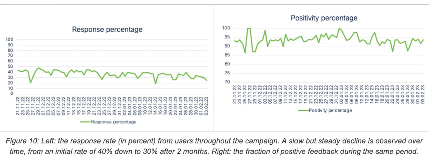
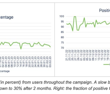
As already mentioned, feedbacks revealing a poor user experience are particularly interesting for modelling, due to their relative rarity compared to positive feedbacks. Figure 10 (right) shows the evolution of the positivity percentage over time. Most feedbacks are positive (consistently over 90%), indicating that QoE degradations are relatively rare events. During the end-of-year shutdown, this fraction increased even further, possibly owing to the larger availability of network resources during this time. The slight drop in positivity in the last 3 weeks is due to a change in the sampling strategy aimed at selecting more negative feedbacks.
Once the feedbacks are ingested, another pipeline runs and associates each feedback with the corresponding telemetry reports. First, all the feedbacks that were shared more than 6 hours after the request are discarded as they are considered outdated. For the remaining labels, each label is matched to the telemetry reports up to 30 minutes prior to the feedback response (as opposed to the feedback request). A study showed that the best matching technique between labels and telemetry reports is with the response rather than the request. An explanation is that users respond based on their recent experience with the application rather than recalling the meeting quality at the time of the request.
The matching technique (one-to-many) described above matches a label to a series of telemetry reports in case the QoE is learned through a time series of KPIs. However, another matching strategy was implemented by matching one label to only one telemetry report (one-to-one). In this scenario, the match happens on the worst telemetry report (in terms of Webex UES) in the last 5 minutes before the feedback collection. If no report is found with this strategy, the corresponding label is discarded in the one-to-one matching dataset. Thus, two datasets can be leveraged for ML purposes depending of the architecture chosen for the model (either tabular data with the one-to-one matching or timeseries in case of one-to-many matching) as described later in this document.
2.4 Training a ML model capable of Predicting the QoE probability
One of the core objectives of Cognitive Networks is to have a highly interpretable QoE model in order to be able to trigger remediation actions. To this end, several models have been trained (and compared) to predict the probability of having positive user feedback from the underlying application KPIs. The probability returned by the model is then interpreted as the QoE score associated with the user telemetry.
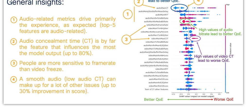
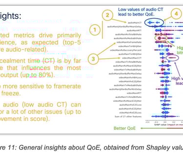
These QoE predictions can be explained using Shapley values to understand which KPI influences the QoE score:
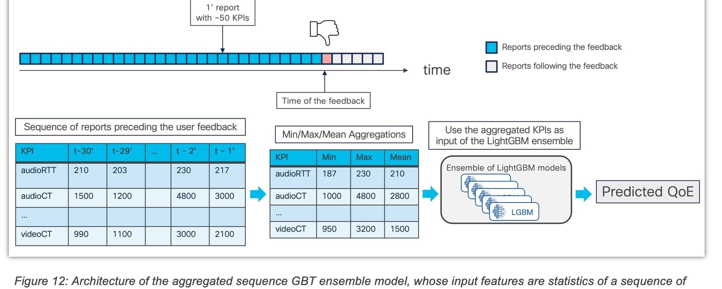
A major improvement in the QoE model performance was obtained by considering a sequence of telemetry reports, rather than one, to predict the user feedback. In the case of the Webex application, each report contains hundreds of KPIs at 1-minute granularity. Therefore, using sequences of reports (e.g., 30 reports) to predict the QoE is quite challenging as it involves leveraging thousands of input features. To solve this problem, two architectures were tested:
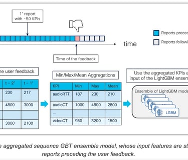
1. An ensemble of GBT models (LightGBM) trained on aggregated KPIs (i.e., the max, min, mean, etc, of each KPI over the sequence of reports).
2. An ensemble of Deep Neural Networks (DNN) featuring an attention mechanism, like the one that is used in Transformers Networks.
We expect the performance of the DNN to be lesser than that of tree-based models, due to the tabular nature of our data[1]. However, as we shall see below, we used a combination of strategies to make these models competitive, albeit not better than trees, while offering opportunities for composability with other differentiable architectures, such as Language Models.
[1] It is indeed a well-known fact that neural networks are vastly outperformed by tree methods on tabular data, especially gradient boosting methods, despite many attempts to the contrary. For a recent survey, refer to Shwartz-Ziv, R., & Armon, A. (2022). Tabular data: Deep learning is not all you need. Information Fusion, 81, 84-90.
2.3 Gradient Boosting Trees (GBT) Models
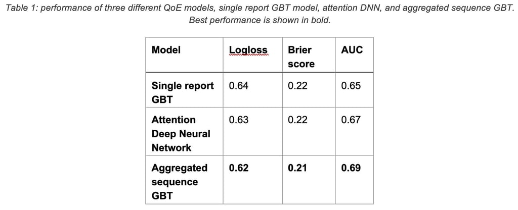
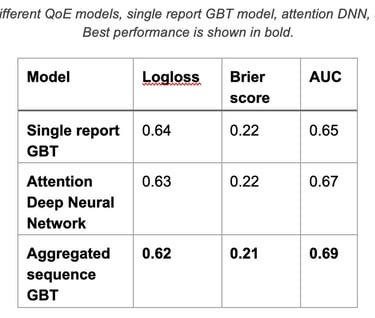
Two variants of Gradient Boosting Trees (GBT) models were used in this study: a single-report model (SRM) and an aggregated sequence model (ASM).
The single-report model is composed of an ensemble of GBT models that were trained using LightGBM on 49 KPIs extracted from a single Webex report. The selection of the specific report is based on a simple heuristic, which involves choosing the report with the lowest Webex UES over the 5-minute period preceding the user feedback. The 49 KPIs encompass Layer 3 metrics such as latency, loss, jitter (end-to-end and hop-by-hop), bitrates (transmitted/received) as well as Layer 7 metrics, such as concealment time, jitter buffer, video resolutions, framerates (requested, received), CPU usage, etc.
To optimize the performance of the model, hyperparameters such as maximum depth, regularization parameters, features, and bagging fractions were fine-tuned. This was achieved through a 10-fold cross-validation process, resulting in the training of 10 GBT models. The number of trees for each model was determined using early stopping. The training process was guided by a Bayesian Optimization strategy, which assessed various combinations of hyperparameters with the 10-fold cross-validation and employed Gaussian Processes to refine the search.
On the other hand, the aggregated sequence model relies on the same set of 49 KPIs used in the single report model. However, instead of extracting the KPIs from a single report, this model aggregates the values of each KPI from the 30 one-minute reports preceding the user feedback. The aggregation process involves calculating the minimum, maximum, and average values for each KPI, resulting in a total of 147 features. The training strategy for the aggregated sequence model follows the same procedure as the single report model, resulting in an ensemble of 10 GBT models.
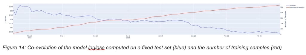
Note: although user feedback must first be gathered to train the models, the process of user feedback collection is not required to once in production. Once the model loss stabilizes, we could see that the model barely improves as additional labels are gathered. Upon reaching such as plateau the model could be released in production, with potential additional campaign of user-feedback collection in the future.
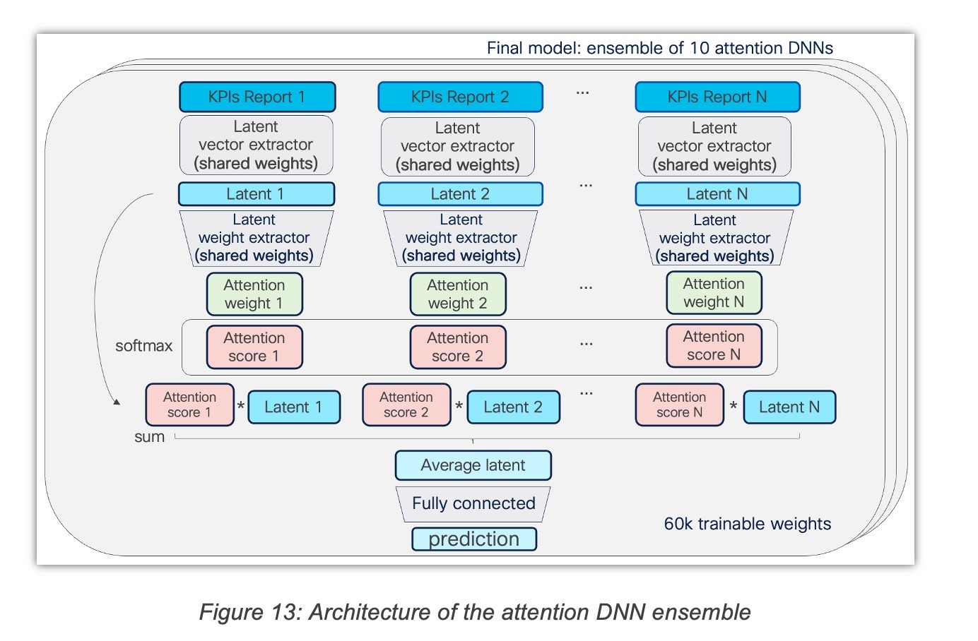
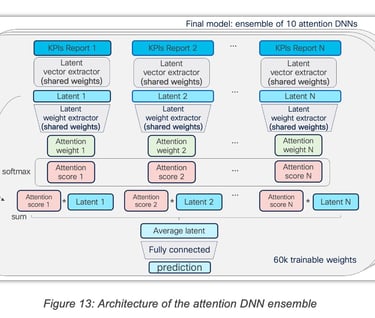
2.6 Attention DNN ensemble architecture
The attention DNN ensemble takes as input sequences of 30 reports (of 49 KPIs) and implements an attention mechanism. Each of the 30 reports is processed by shared feed-forward layers that produce latent vector “values” and a latent score for each report. Then, the softmax activation is applied to the scores, and each “values” vector is multiplied by its corresponding softmaxed attention score. We use the "SELU" (Scaled Exponential Linear Unit) activation for all the dense layers, except the last dense layer that uses a "sigmoid" activation.
2.6.1 Normalization of the KPIs
The normalization of the KPIs had a massive impact on the performance of the QoE attention DNN. The normalization that led to the best results consists in applying quantile discretization to each KPI (with ~100 quantile values). This way, ~100 bins (categories) are created for each KPI. Then, each category is encoded by an embedding that is learned during training.
2.6.2 Dealing with missing values
Quite often, the telemetry reports miss some KPI values. Since the DNNs cannot natively deal with missing values (contrary to GBT), these missing values need to be encoded to be processed by the DNN. To solve this, for each KPI, a special category for the missing values was created during the discretization process detailed above.
2.6.3 Skip connections
To prevent the vanishing gradient issue, concatenated skip-connections were employed. This technique consists in providing a given dense layer with intermediate representations, in addition to the representation computed by the previous dense layer. This allows the intermediate representations to flow across the entire network, even when it is very deep.
2.6.4 Bagging of LGBM models
Early stopping was used to avoid overfitting. Instead of training one model with one train/validation split (which results in sacrificing a significant part of the training dataset to create the validation set), 10 models were trained in a 10-fold cross-validation. The resulting ensemble model is obtained by averaging the predictions of the 10 models. The same bagging process is used for the aggregated sequence GBT and the single report GBT models.
The following table compares the performance of the two QoE sequence models and the single report model:
2.7 Results of learning complex patterns
Assessing the Quality of Experience (QoE) of an application requires considering numerous network and application KPIs, which can vary over time. As hinted by the previous result (sequence models outperform single report models), time plays a crucial role in this process as even minor disruptions can be aggravating for the user when they accumulate over time. For example, consider a video-conferencing application: QoE can be easily assessed to be poor when a user encounters a clear disruption, such as losing all connectivity to the media server for 30 seconds. However, frequent short audio or video glitches can also lead to a poor QoE, even if each individual incident is short and minor. Such phenomenon has been studied in the context of VoIP years ago where it was shown that the number of disruptions due to traffic reroutes (even when falling back to the most optimal path) had to be minimized. In other words, the patterns of disruption along with their nature play a critical role in terms of user experience.
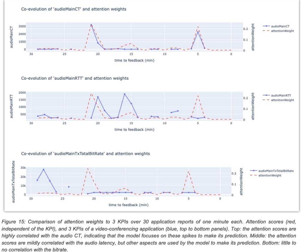
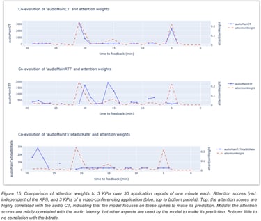
One benefit of the attention DNN model is the interpretability of the latent attention scores computed at inference time. Indeed, the structure of the attention model forces it to focus more on the reports having the greatest attention score to predict the QoE. Therefore, the greater the attention score of the report, the greater its contribution to the QoE.
Extracting the sequence of attention scores at inference time provides a method to identify the failure mode of an application session, as it projects a multi-dimensional sequence of KPIs onto a one-dimensional sequence. As a result, it allows for instance to distinguish between a poor QoE caused by a single local disruption (reflected by a single peak of attention) or by an accumulation of slightly annoying moments (in which case the attention is diluted over multiple reports).
The example shown in Figure 8 demonstrates a sequence of 30 reports where the model focused mostly on two specific moments where the user had a very high value for a video conferencing KPI audioMainCT (audio concealment time), resulting in a correct prediction of the QoE.
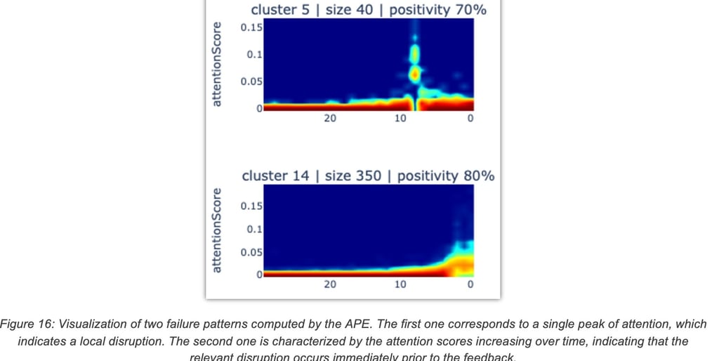
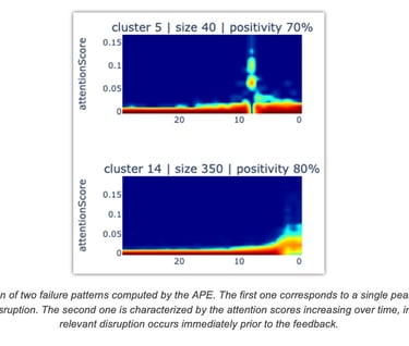
In an initial effort to identify temporal failure patterns, the attention DNN was applied to the collected dataset (telemetry and user feedbacks) to extract a sequence of attention scores for each sample. Then, a sequence clustering algorithm (time-series K-means) was used to group the attention scores into clusters. Each cluster can be visualized by plotting a heatmap of the attention score sequences it contains, as shown in Figure 16.
2.8 Specific Performance Metrics for QoE Models
QoE models are used to detect situations that lead to poor user experience (QoE). To this end, we rely on feedbacks from these users about their experience using the application at a given time T. Such feedbacks are then used to train a model in charge of predicting the QoE.
Because user ratings are intrinsically subjective and noisy, we do not actually care about individual outcomes, but statistics thereof. Our assumption is that, given a situation X, if user A provides a positive label and user B provides a negative label, this might be due to:
1. Subjectivity biases: user A may consider the experience acceptable because the audio is excellent, while user B is unhappy because the video resolution is lower than usual. Obviously, such differences are important and could be learned if we provided the model with details about the user’s focus. In absence thereof, such contradictions appear as random (noise). Said differently, the criterion for users A and B for assessing the user experience are simply different. Note also that the same user A may even sometimes provide inconsistent feedback (different feedback under similar conditions) due to intrinsic human subjectivity.
2. Differences in understanding: in the same situation as before, user B may be unhappy because he had trouble joining the meeting. While this is a valid cause of dissatisfaction, our QoE model is not designed to capture such aspects and such contradictions will again appear as random.
3. Incorrect feedback: user B may simply have clicked on the wrong button or maliciously provided contradictory feedback.
All the above factors require us to rely on probabilistic metrics, which do not consider individual outcomes, but rather statistics thereof. In a nutshell, we do not measure the ability of the model to predict whether a given sample is positive or negative, but rather its probability of being positive (or negative).
2.8.1 Issue detection: the retrieval problem
Detecting issues is akin to the problem of information retrieval, wherein one uses a system (e.g., a search engine) to retrieve a set of results from a database. The key metrics in this area are those of precision and recall. Now, such metrics can only be computed for a given threshold. Alternatively, one can measure the so-called gain of a given model w.r.t. a baseline (e.g., a random retrieval) across a plurality of thresholds.
Let us consider the following scenario. Given a dataset of samples, we use a model to retrieve those samples that were rated “bad QoE” by the users. We then ask the following question, what is the precision and recall obtained by retrieving the N samples with the lowest predicted QoE, given different values of N? As we vary N, the expected precision and recall might change: if N is larger than the total number of negatives, the precision can never be 1.0, as we will necessarily retrieve some positives. Conversely, if N is smaller than the total number of negatives, the recall can never be 1.0.
However, setting the value of N to the total number of negatives in the dataset causes the precision and the recall to be equal: each negative retrieved contributes to increasing both the precision and the recall by the same amount. We call this value the Negative Retrieval Accuracy (NRA), and it is given by
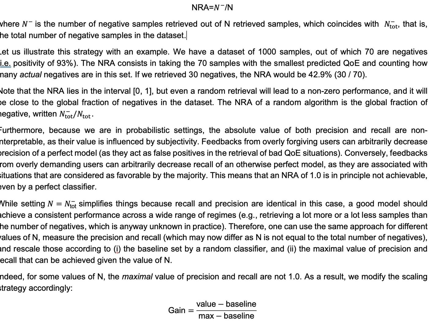
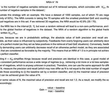
This strategy is identical whether we compute a precision or recall gain. The value of max and baseline are set based on the value of N, which determines the upper bound of the value and the baseline of a random sampling strategy, respectively. All these values can be computed analytically using basic probability theory. For instance, if value is a recall and the number of retrieved samples N is only half of the total number of negatives, then max is set to 0.5 and baseline is set to . If value is a precision and the number of retrieved samples N is twice the total number of negatives, then max is set to 0.5 and baseline is set to the global fraction of negatives.
Finally, we report the so-called Precision Recall Gain (PRG), which is the average gains of precision and recall across a set of values for N, e.g. corresponding to regular fractions of the total sample size between 2.5% and 50%.
For the sake of illustration, let us draw the Precision Recall Curve (PRC) for our model ens10 and the Webex UES, both in their calibrated and natural variants:
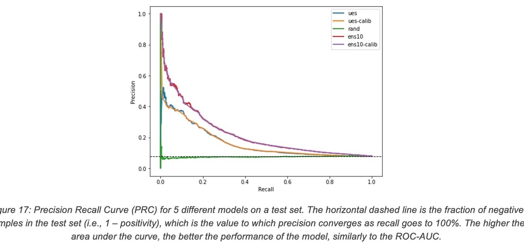
One can clearly see from this curve that our models exhibit a significant lift, but a precision above 80% is essentially impossible to achieve (in that regime, the Webex UES has a recall of 0% while our models have a recall of 1%). Even a precision of 50% is not achievable by the UES with a non-zero recall, while our models achieve a recall of 8%.
2.8.2 Decision making: the Bipartite Ranking problem
When one wants to use a model for decision-making, the calibration of predicted probabilities is not very important. Instead, the critical aspect is whether the model predictions induce a correct ordering over the samples, i.e., the higher the prediction, the higher the frequency of positive outcomes. This problem is referred to as Bipartite Ranking in the literature, and it can be more formally described as maximizing the area under the ROC curve.
A classical measure of performance for ranking algorithms is the so-called empirical ranking error, which is the fraction of positive-negative pairs that are ranked incorrectly by the model, i.e. a higher probability is assigned to the negative sample than to the positive sample, wherein ties are broken at random uniformly. The empirical ranking error is equal to one minus the area under the ROC curve (AUC) (see Agarwal, Shivani. “A study of the bipartite ranking problem in machine learning.” University of Illinois at Urbana-Champaign, 2005). Indeed, although it is not obvious from its formulation, the AUC of a model is the probability that a randomly drawn positive is assigned a higher score than a randomly drawn negative, which is an intuitive interpretation (see Menon et al., “Bipartite ranking: a risk-theoretic perspective.” The Journal of Machine Learning Research 17.1 (2016): 6766-6867).
For instance, imagine we have the following dataset, ordered by decreasing predictions:
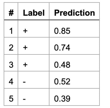
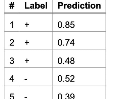
We have 3 positives and 2 negatives, and therefore 6 pairs of samples with opposite labels to consider. Out of those, 5 pairs are correctly ordered (i.e. the negative sample is assigned a lower prediction than the positive sample), but one pair is incorrectly ordered (i.e. the pair (3, 4)). In this example, the empirical ranking error is 16.7% (1/6) and the AUC is 83.3% (5/6).
2.8.3 Visibility: the Reliability-Resolution tradeoff
We are particularly interested in the following tradeoff, which is a well-established effect in probabilistic classification:
1. Reliability: the accuracy of predicted probabilities w.r.t the true frequency of positive outcomes. This can be almost trivially achieved by a constant classifier, which always predicts the global rate of positive samples in the training set, which is the average rate of positive labels in the training dataset. While a model that does this may score relatively high in terms of reliability, it has no practical use since the model always predicts the same value regardless of the underlying scenario. Based on the sheer number of labels that we have accumulated; the overall positivity lies around 93%.
2. Resolution: the variance of individual predictions, which indicates whether some information is captured by the model. The constant classifier described earlier will achieve zero resolution, as there is no information whatsoever in its predictions (since they are constant).
Let us illustrate this tradeoff with an example. Assume that we have two groups of samples with the same size but different positivity. The first group has a positivity of 86% and the other group has a positivity of 100%. Hence, the overall positivity is 93%. A model that predicts always 0.93 for every sample would achieve a perfect reliability, but zero resolution as its predictions have no variance. A much superior model would be one that correctly predicts 0.86 for the first group and 0.93 for the second: this model would have the same reliability, but a much-increased resolution.
In other words, we aim at achieving the highest resolution without sacrificing too much reliability. Note that this tradeoff is quite similar to the precision-recall found in the area of information retrieval or sensitivity-specificity used in medical diagnosis, where increasing one leads to a reduction of the other.
The Brier score captures exactly this tradeoff: Brier = Reliability - Resolution + Uncertainty
where Uncertainty is a term correlated with the total entropy of the dataset, which does not depend on the model predictions. It can be thought of as a measure of the “difficulty” of the problem. See this article for further details about the 3-component decomposition of the Brier Score.
The issue with the Brier Score is that a model with a zero resolution may still achieve a relatively high score, although such models have no practical value and one might be absolutely willing to sacrifice some reliability so as to achieve non-zero resolution. This is the reason why the Brier Score is often considered difficult to interpret and why constant models are difficult to beat by a large margin on this metric.
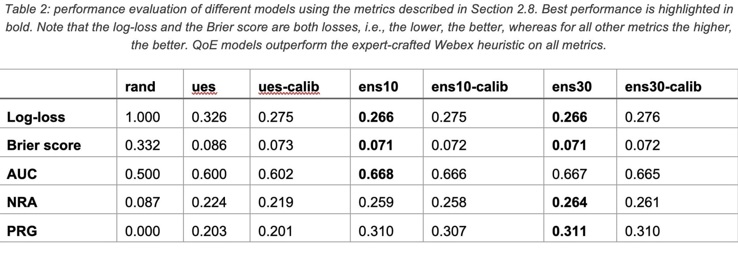
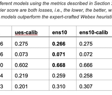
2.8.4 Quantitative results from QoE models
Table 2 provides an overview of the performance of different models across all metrics described earlier. The models represented in the table are:
Random classifier (rand): a random baseline, which yields a random score uniformly distributed between [0, 1]. This serves as an experimental control.
Webex UES (ues): the Webex UES, which is a 1-5 score, rescaled to be in the interval [0, 1]. We also consider a calibrated variant (ues-calib), which uses an isotonic regressor as calibrator.
Ensembles of Gradient Boosting Trees (see Section 2.5 for details), denoted ens{n-trees}, of different sizes (10 and 30) and calibration or not.
The key takeaways from this study are the following:
1. The log-loss or Brier score have extremely limited variability, although other metrics vary more significantly. Models outperform the Webex UES on all metrics.
2. The NRA values remain low even for the best models, peaking at 26.4%. While this may seem poor, we must remember that the overall negativity of the dataset is only of 7.7% and a perfect model may achieve a NRA anywhere between 28.4% and 100%, depending on the Bayes error rate.
3. The lift between the Webex UES and the best models is quite modest on the NRA (22.4% vs 26.4%), but significantly larger on precision/recall gains (20.3% vs 31.1%). This indicates that our models have a more consistent behavior across the entire range of predictions.
2.9 Multi-Application Models (MAM) and Transfer Learning
The issue of learning generalization is one of the most challenging tasks with machine learning. When a ML algorithm is trained for a task A, could one easily apply the learning to a “similar” task using “similar” input? A number of approaches have been proposed to that end such as domain adaptation and transfer learning. As discussed in (Vasseur J. , AI and Neuroscience: the ( incredible ) promise of tomorrow, 2023), learning generalization in AI could greatly benefit from our understanding of the brain learning mechanisms.
Domain adaptation refers to the process of using a model on a new (target) domain for which input features have a different distribution than the set of input features used to train in the original domain (also called the source domain). Domain adaptation does not refer to a specific technique and many approaches have been proposed such as using normalization, weighting or even learning a transformation in order for the distribution between source and target domain to look alike. Instance level adaption is an approach where instance in the source domain are re-weighted to be more representative of the target domain; model adaptation consists in fine-tuning the model using a small dataset from the target domain. Note that in the Large Language Model (LLM) domain, domain adaptation is performed using PEFT (Parameter Efficient Fine Tuning) with techniques such as LoRA (Low Rank Adaptation) where a model trained with a given (large) dataset may be fine-tuned using a smaller dataset from a target source.
Transfer Learning refers to a very common model adaptation technique that aims to re-use a model trained for a task A and apply it to a “similar” task B. It is worth noting that the major challenge is to train the model for a new task B without degrading the performance for task A, a common challenge referred to as “Catastrophic Forgetting”. Various approaches exist to mitigate such an issue such as multi-task learning or even using a per-task specific subset of weights such as with LoRA.
In our case, the idea is to re-use the model trained for QoE probability prediction trained using cross-layer variables including a rich set of Webex variables and determine how to apply it to other conferencing applications such as Microsoft Teams and Zoom?
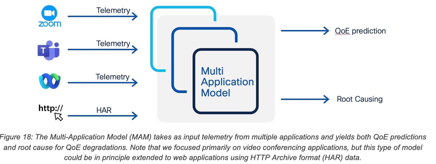
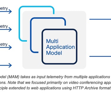
The Multi-Application Model (MAM) was studied for the class of video conferencing applications Webex, Zoom and M365 Teams. The goal of the study was to understand if a QoE model trained on one application’s telemetry could be efficiently used to predict the QoE for another application. Voice and video calls were generated for each collaboration application using the same set of network impairment scenarios and the resulting voice and videos recordings were then used to collect user-experience feedback through the AWS Mechanical Turk (MTurk) data labeling service, reusing the methodology described in Section 2.2.
Performance telemetry for each conferencing application was retrieved from its respective vendor performance monitoring dashboard and records for each of the network impairment scenarios along with the average acceptance score was computed. Zoom application telemetry was retrieved from the Zoom Metrics Dashboard using 1-minute granularity. For M365 Teams, we retrieved Call Analytics telemetry with a 10-second granularity using the Team Admin Center tool. For Webex, telemetry was retrieved using the previously described streaming mechanism at 1-minute granularity.
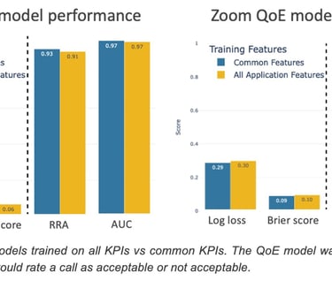
Acceptance score is the indicator that shows whether the user found the quality of the call acceptable or not (binary feedback). The average acceptance is computed over all the user feedback collected for a particular impairment scenario and is shown in Figure 19.
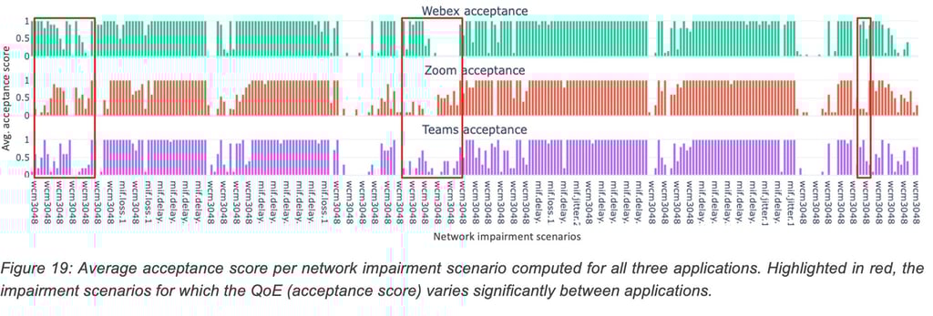
Figure 19 shows the variation in the user acceptance score between applications for the same underlying network conditions. This shows that QoE is application specific for some scenarios and a QoE model does indeed require some form of domain adaptation to predict accurate QoE for a new application.
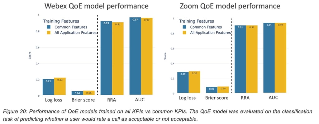
Apart from the varying application behavior for similar network conditions, the difference in the set of KPIs available through the telemetry add to the challenge of developing a multi-application model. While some of the KPIs such as frame-rate, CPU usage, bit rate are commonly available across applications, other useful KPIs such as concealment time, buffer delay, etc., are sometimes application-specific and only available for one of the applications. Using only the common KPIs for the sake of a common model may impact the QoE model performance as we might exclude some important signal contained in an application specific KPI. To understand the loss of information by excluding the application specific KPIs, we performed an ablation study, where we compared the QoE model (single application) performance when only the common KPIs are used versus when all available KPIs are used in predicting the QoE. It can be shown that performance did not degrade much when only the common KPIs were used. It is to be noted that the test set only consisted of telemetry corresponding to the lab generated impairments. Real world scenarios may contain important signals within application-specific telemetry.
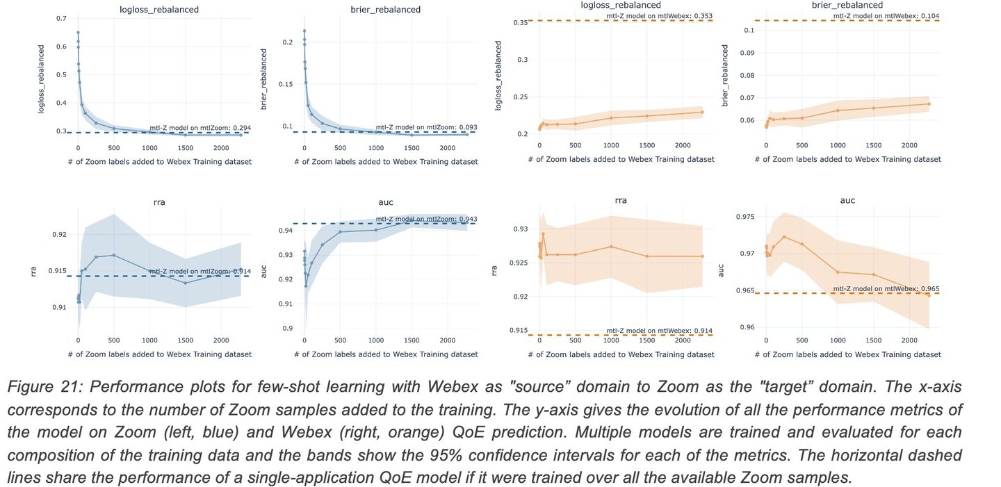
To understand the feasibility of a multi-application model, a QoE model trained on a “source” application (Webex) is iteratively trained with samples from a different "target” application (Zoom). We then study the change in the QoE prediction performance for the target application as we increase the number of samples from the target domain. This few-shot learning study shows whether there is a meaningful increase in performance for the target application, without decrease in performance for the source application. Figure 21 depicts the change in performance on both Zoom and Webex with an increasing number of samples from the target domain (Zoom). Note how a few samples (< 500) allow the model to achieve nearly the same performance as with the entire dataset (horizontal line).
3. Can we make the network QoE-driven and self-healing?
Traditional Network Design and Planning: This process has traditionally been a long-term loop. Initially, the network is designed based on "rough" predictions of future application deployments, traffic demands, and a set of expected quality metrics, all of which being loosely connected. Various tools can then compute an optimized topology (and a set of routing metrics) to meet constraints, such as maximum average/peak load per link or maximum end-to-end delays. This is followed by SLA measurements using an array of tools. If any constraint is not met or an unforeseen one arises (like traffic growth), the cycle restarts.
Dynamic control planes have been designed to adjust path computation to meet network-centric SLAs, such as in MPLS Traffic Engineering. Here, Traffic-Engineering Label Switched Paths (TE LSP) may be used and computed using distributed CSPF or The Path Computation Element (PCE) in order to perform constrained-based routing for some traffic having specific requirements. Similar concepts are also employed in Segment Routing (SR). In context of enterprise networks, SD-WAN features such as Application Aware Routing (AAR) look to optimize the best path between sites by selecting or excluding overlay tunnels based on loss, latency, and jitter SLA profiles. Low granularity measurements of Delay, Loss and Jitter can then be used to redirect traffic when it is determined than the current path does not meet the current SLA (specified using hard thresholds on the networking KPI values).
In all the examples above, QoE is tied to network-centric SLA such as delay, loss and jitter, using hard (and poorly) defined constraints.
In contrast, Cognitive Networks leverage the ability to compute/infer QoE and then activate automation actions to continually optimize the network for QoE, not just network metrics such as link load or delays. But why? As outlined in previous sections, QoE is more intricate than merely meeting hard-coded bounds for delay, jitter, and loss and must be learned using ML algorithms. While dynamic methods can optimize and adhere to network metric constraints, optimizing a network where QoE is influenced by ML learning requires a new approach.
To this end, we are introducing a novel self-healing method for Cognitive Networks using ML to learn QoE coupled with a suite of tools for network automation to optimize the estimated (and learned) QoE.
Which tools could be used by Self-Healing network to optimize QoE? A myriad of automation tasks could be triggered, here are a few examples:
· Dynamic QoS: Technologies in networks enabled with QoS often involve traffic marking, queuing, various congestion avoidance mechanisms like (W)RED, and even traffic shaping. These mechanisms typically adhere to static templates and are infrequently adjusted, primarily due to the unpredictable effects of such changes.
· Path Change in the Internet Using Loose Hop Routing: It might not always be feasible to directly influence a path on the Internet, but different "backbones" can be utilized. For instance, for traffic directed to a SaaS application, an SD-WAN deployment might choose an MPLS or Internet tunnel back to a Data Center (DC) or a Direct Internet Access (DIA) path. With a given DIA, the path determined by BGP might be followed, or the traffic might be rerouted to a gateway of another hyperscaler, such as Google, Azure, or AWS.
A potential implementation might use the QoE model to evaluate QoE, followed by another learning algorithm to enhance it. Techniques like Shapley values could root-cause QoE by determining which input features influence it. Based on feature importance, actions could be triggered, and their QoE impact measured, and possibly improved using for example Reinforcement Learning. Cognitive networks might employ Differentiable Programming (a generalization of Deep Neural networks). This approach could optimize user satisfaction (QoE) using multi-layer telemetry, which would predict QoE and activate networking actions. Though these components aren't new in isolation, the capability of a system to genuinely assess and optimize QoE is groundbreaking and will likely be pivotal for future networking.
With the advent of Software Defined Cloud Interconnect (SDCI) and Middle Mile Optimization (MMO), networks can be provisioned on-the-fly. Today, while APIs can create such networks, there aren't tools that offer insights on optimal topologies and resources needed to maximize variables like user QoE. Cognitive networks could dictate the actions required for such objectives, representing a fundamental shift in network operations.
Here are two real world examples illustrating how Cognitive Networks have been be used to model QoE and then take actions to improve it:

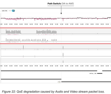
The first example (Figure 22) shows a Cognitive Networks dashboard for a Webex user in Lisbon, Portugal. The first row of metrics corresponds to the QoE scored as inferred by a ML model, while the following rows list the Webex application metrics in order of feature importance (as per Shapley values inspection).
For the first half of the graph, in what we could call the default state, the user audio/video traffic travels over a DIA link (public internet) to the closest Webex data center located in London UK. We notice that during this period, the QoE score experiences frequent and significant drops which can be correlated with degradations of audio and video packet loss metrics.
Halfway through, a new overlay path is instantiated from the user location to an AWS PoP and traffic is rerouted on the new path. Using the new path Webex traffic from the user travels first to AWS PoP in Paris, France after which it uses the AWS backbone to reach the Webex data center in London, UK. After the change is implemented, we see the packet loss spikes disappear and the QoE score stabilizes.
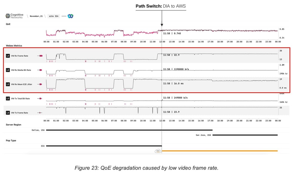
The second example (Figure 23) shows the same dashboard for a Webex user in Mexico City, Mexico. In the default state (first half of the graph) Webex traffic flows from the user to Webex Data Center in Dallas, USA directly over the internet (DIA) and experiences several periods of major degradations. The system flags several application metrics (layer 7) related to the incoming video stream (frame rate, bit rate, mean jitter) as the main culprits.
Similarly to the previous example, halfway through user traffic is rerouted to an alternate path via the AWS PoP in San Francisco. Following the reroute, even though the new path is longer from a distance and latency perspective, we see the previously highlighted video metrics stabilize and the QoE score remains consistently high.
3.1 Inventing a new Layer-7 signaling control plane for applications
According to the principle of "layer" isolation, one might not anticipate the lower layers of the renowned layer stack to receive signals from the upper (application) layer. This layer isolation has prompted application teams to address application layer issues and then potentially relay to lower-layer teams to investigate the root cause. As highlighted in this paper, adopting a cross-layer holistic approach—where application feedback is combined with lower-layer telemetry to train a ML model can enhance our understanding of QoE determinants, identify potential root causes, and even drive network automation.
But how can a system automatically collect application feedback? Several ad-hoc solutions have been implemented, as seen in collaborations between Cisco and Microsoft, where cloud-based APIs were developed to allow networking controllers to gather user feedback in the form of discrete labels describing per-application estimated user experience. This isn't as granular as feedback directly from users, however. As already pointed, gathering user feedback used to train model may be done sporadically.
Still an approach consisting in gathering user feedback using a standardized application signaling protocol, allowing applications to provide feedback using both discrete and continuous variables at varying levels of granularity and aggregation would be highly beneficial.
4. Conclusion
For the past few decades applications and networking teams have been debating on why users may complain about poor experience, with the objective of finding the “root cause” and supposedly fix it, always in reactive mode.
Although undeniable advancements have been made in every facet of networking—providing more bandwidth, ensuring smoother experiences, and achieving higher reliability— one must admit that our understanding of QoE (Quality of Experience) has lagged. Even though this understanding might be the key to improving the true user experience and adjusting the network accordingly, traditional approaches have merely set hard boundaries for network-centric variables (specifically delay, loss, and jitter). These boundaries are measured using vaguely defined frameworks to meet the required SLAs.
In this experiment, we adopt a radically different and novel approach. We gathered real-time binary user feedback alongside a comprehensive set of cross-layer telemetry variables for voice/video applications. These were then used to train a machine learning (ML) algorithm capable of inferring the true user experience (aka QoE). Analyzing this model offers profound insights into the actual root causes. More crucially, it reveals intricate patterns that more accurately depict what influences QoE. As demonstrated in this paper, this method is far superior to the traditional threshold-based approaches previously employed.
Undoubtedly, such an approach necessitates collecting a vast amount of user feedback. But would this be feasible given the thousands of applications out there? Firstly, not all applications demand a profound understanding of QoE; only those with strict SLAs do. Secondly, with the advent of sophisticated ML/AI algorithms capable of model adaptation, this approach would be constrained to a few, albeit critically important, classes of applications. Lastly, as mentioned earlier, this could pave the way for the development of application signaling protocols designed to gather user feedback, which in turn would be utilized to train ML/AI algorithms for QoE comprehension.
Moreover, Cognitive Networks could pave the way for the long-awaited Self-Healing Networks. These networks would auto-adjust using the predicted QoE and make use of a set of adjustment parameters (like QoS, routing, topology, etc.) in order to constantly optimize and recalibrate for improved user experience. For the first time, we might witness the emergence of a truly QoE-driven self-healing network.